Fine-mapping with susie accounting for kinship
Table of Contents
Introduction
The susie model (Wang et al. 2020) for statistical fine mapping is \( \DeclareMathOperator\Mult{Multinomial} \DeclareMathOperator\N{\mathcal{N}} \newcommand\mi{\mathbf{I}} \newcommand\mk{\mathbf{K}} \newcommand\mh{\mathbf{H}} \newcommand\ml{\mathbf{L}} \newcommand\mx{\mathbf{X}} \newcommand\vb{\mathbf{b}} \newcommand\vgamma{\boldsymbol{\gamma}} \newcommand\vpi{\boldsymbol{\pi}} \newcommand\vtheta{\boldsymbol{\theta}} \newcommand\vy{\mathbf{y}} \)
\begin{align} \vy \mid \mx, \vb, \sigma^2 &\sim \N(\mx\vb, \sigma^2 \mi)\\ \vb &= \sum_{l=1}^L \vgamma_l \beta_l\\ \beta_l \mid \sigma^2_l &\sim \N(0, \sigma^2_l)\\ \vgamma_l \mid \vpi &\sim \Mult(1, \vpi). \end{align}In this model, the multiple regression effect vector \(\vb\) is assumed to be a sum of single independent effects \(\vgamma_l \beta_l\). The posteriors \(p(\vgamma_l \mid \mx, \vy, \vtheta)\), where \(\vtheta = (\sigma^2, \sigma_1^2, \ldots, \sigma_L^2)\), can be approximately estimated by variational empirical Bayes and interpeted as credible sets, each with some minimum posterior probability of containing (at least) one causal variant.
Under this model, residuals are assumed to be independent; however, this assumption may not hold when individuals are related to each other or when there is substantial population structure among individuals. To address this issue, it is common (reviewed by Yang et al. 2014) to instead assume that
\begin{align} \mh &\triangleq \sigma^2_u \mk + \mi\\ \vy \mid \mx, \mh, \vb &\sim \N(\mx\vb, \sigma^2 \mh), \end{align}where \(\mk\) denotes the kinship matrix or genetic relationship matrix. Under this more complex model, residuals are correlated due to relatedness (shared genotypes) between individuals.
Modifying the existing inference algorithm for the susie model to incorporate this more complex likelihood may be cumbersome (particularly, estimation of \(\sigma_u^2\)). Here, we instead pursue a simpler approach based on the whitening transform
\begin{align} \ml\ml' &\triangleq \mh^{-1}\\ \tilde{\mx} &\triangleq \ml\mx\\ \tilde{\vy} &\triangleq \ml\vy\\ \tilde{\vy} \mid \tilde{\mx}, \vb &\sim \N(\tilde{\mx} \vb, \sigma^2\mi). \end{align}The key idea of this approach is that, for fixed \(\sigma_u^2\), the more complex problem reduces to a simpler susie problem. As a result, one can use the existing inference algorithm as a subroutine in a procedure that additionally estimates \(\sigma_u^2\).
Setup
import functools as ft
import numpy as np
import pandas as pd
import scipy.optimize as so
import scipy.linalg as sl
import txpred
import rpy2.robjects.packages
import rpy2.robjects.pandas2ri
rpy2.robjects.pandas2ri.activate()
susie = rpy2.robjects.packages.importr('susieR')
%matplotlib inline
%config InlineBackend.figure_formats = set(['retina'])
import colorcet
import matplotlib.pyplot as plt
plt.rcParams['figure.facecolor'] = 'w'
plt.rcParams['font.family'] = 'Nimbus Sans'
Methods
Considerations for estimation
One immediately apparent issue is that inference after the whitening transform yields approximate posteriors \(p(\vgamma_l \mid \tilde{\mx}, \tilde{\vy}, \vtheta)\), where \(\vtheta = (\sigma^2, \sigma_u^2, \sigma_1^2, \ldots, \sigma_L^2)\), when the target posterior was \(p(\vgamma_l \mid \mx, \mh, \vy, \vtheta)\). However, fixing \(\vtheta\),
\begin{align} p(\vgamma_l \mid \tilde{\mx}, \tilde{\vy}, \vtheta) &= \frac{\int p(\tilde{\vy} \mid \tilde{\mx}, \vb, \vtheta) p(\vgamma_l \mid \vtheta)\, dp(\beta_l, \vb_{\setminus l} \mid \vtheta)}{\int p(\tilde{\vy} \mid \tilde{\mx}, \vb, \vtheta)\, dp(\vb \mid \vtheta)}\\ &= \frac{(1 / \det(\ml)) \int p(\vy \mid \mx, \mh, \vb, \vtheta) p(\vgamma_l \mid \vtheta)\, dp(\beta_l, \vb_{\setminus l} \mid \vtheta)}{(1 / \det(\ml)) \int p(\vy \mid \mx, \mh, \vb, \vtheta)\, dp(\vb \mid \vtheta)}\\ &= p(\vgamma_l \mid \mx, \mh, \vy, \vtheta), \end{align}where the integrals are over the remaining factors of the prior in the numerator, and over the entire prior in the denominator.
Remark. This argument relies critically on fixing \(\sigma_u^2\); therefore, there are likely many complications if one assumes a prior distribution on \(\sigma_u^2\).
The next issue that arises is estimation of \(\vtheta\). The ELBO before the whitening transform contains a term \(-\frac{1}{2}\ln\det(\mh) = \ln\det(\ml)\) that vanishes after the transform. Therefore, for fixed \(\sigma_u^2\) (i.e., fixed \(\ml\)), one can use the existing algorithm to maximize the ELBO with respect to the remaining components of \(\vtheta\) (since the term that is left out of the ELBO corresponding to the transformed problem does not depend on those components). Thus, there are a few ways one could produce a point estimate of \(\sigma_u^2\):
- The easiest way is to first estimate \(\sigma_u^2\) e.g., by REML, and then simply whiten the data once.
- A slightly more complex approach is to use a line search procedure, e.g., Brent's method, to maximize the ELBO over \(\sigma_u^2\), at each candidate value maximizing the ELBO using the existing algorithm as a subroutine on candidate whitened data.
Remark. Since susie estimates \(\sigma^2\), some care is likely needed in handling scaling of \(\mx, \vy\).
Of course, the most complex approach would be to modify the single effect regression subroutine underlying the existing algorithm to account for \(\sigma_u^2 \mk\). The advantage of the simpler approaches is that they do not require modifying the existing algorithm; they simply use the existing method as a subroutine.
A final issue is estimation of \(\mk\) itself (in the absence of pedigree information). Listgarten et al. 2012 discuss a potential loss of power due to proximal contamination: double-counting the effects of the cis-genotypes \(\mx\) in the design matrix and the residuals. They recommend estimating \(\mk\) using SNPs on chromosomes other than the one containing the cis-genotypes of interest.
Implementation
Here, we prototype the simple approaches described above.
def unwhiten(K, su):
  assert su >= 0
  H = su ** 2 * K + np.eye(K.shape[0])
  W = sl.cholesky(H)
  return W

def whiten(K, su):
  assert su >= 0
  H = su ** 2 * K + np.eye(K.shape[0])
  W = sl.cholesky(sl.pinv(H))
  return W

def susie_kinship_loss(su, x, y, K, **kwargs):
  print(f'fitting su={su:.12g}')
  W = whiten(K, su)
  fit = susie.susie(W @ x, W @ y, **kwargs)
  # -1/2 log(det(H)) = log(det(W))
  return -fit.rx2('elbo')[-1] - np.log(sl.det(W))

def susie_kinship(x, y, K, su=None, bounds=None, **kwargs):
  if bounds is None:
    # TODO: these bounds may not work depending on scaling
    bounds = [0, 10]
  if su is None:
    f = ft.partial(susie_kinship_loss, x=x, y=y, K=K, **kwargs)
    fit0 = so.minimize_scalar(f, bracket=[0, 1], bounds=bounds, method='bounded')
    if not fit0.success:
      raise RuntimeError('failed to estimate su')
    su = fit0.x
  if su < 0:
    raise ValueError(f'invalid value of su ({su})')
  W = whiten(K, su)
  fit = susie.susie(W @ x, W @ y, **kwargs)
  return fit
Results
Simulated example
Read genotypes of all individuals (including Yoruba in Ibadan, Nigeria; YRI) in cis of the top eQTL called in European samples collected by GEUVADIS.
sbatch --partition=mstephens --mem=4G
#!/bin/bash
module load htslib
module load plink
tabix -h /project2/compbio/geuvadis/genotypes/GEUVADIS.chr6.PH1PH2_465.IMPFRQFILT_BIALLELIC_PH.annotv2.genotypes.vcf.gz 6:$((86388451-500000))-$((86388451+500000)) | gzip >/scratch/midway2/aksarkar/txpred/geuvadis/ENSG00000203875.4.vcf.gz
plink --memory 4000 --vcf /scratch/midway2/aksarkar/txpred/geuvadis/ENSG00000203875.4.vcf.gz --maf 0.01 --geno 0.01 --hwe 0.05 --make-bed --out /scratch/midway2/aksarkar/txpred/geuvadis/ENSG00000203875.4
x = txpred.dataset.read_plink('/scratch/midway2/aksarkar/txpred/geuvadis/ENSG00000203875.4')
xs = x.values - x.values.mean(axis=0, keepdims=True)
xs /= x.values.std(axis=0, keepdims=True)
xs.shape
(465, 3509)
LD prune the GEUVADIS genotypes to compute the GRM.
sbatch --partition=mstephens --mem=4G -a 1-21%4
#!/bin/bash
module load plink
plink --memory 4000 --vcf /project2/compbio/geuvadis/genotypes/GEUVADIS.chr${SLURM_ARRAY_TASK_ID}.PH1PH2_465.IMPFRQFILT_BIALLELIC_PH.annotv2.genotypes.vcf.gz --maf 0.01 --geno 0.01 --hwe 0.05 --indep-pairwise 500 10 0.1 --make-bed --out /scratch/midway2/aksarkar/txpred/geuvadis/chr${SLURM_ARRAY_TASK_ID}
plink --memory 4000 --bfile /scratch/midway2/aksarkar/txpred/geuvadis/chr${SLURM_ARRAY_TASK_ID} --extract /scratch/midway2/aksarkar/txpred/geuvadis/chr${SLURM_ARRAY_TASK_ID}.prune.in --make-bed --out /scratch/midway2/aksarkar/txpred/geuvadis/pruned-chr${SLURM_ARRAY_TASK_ID}
Estimate the GRM.
sbatch --partition=mstephens --mem=4G
#!/bin/bash
module load plink
parallel echo /scratch/midway2/aksarkar/txpred/geuvadis/pruned-chr{} ::: $(seq 1 22) >pruned-geuvadis-merge.txt
plink --memory 4000 --merge-list pruned-geuvadis-merge.txt --make-rel square bin --out /scratch/midway2/aksarkar/txpred/geuvadis/pruned-geuvadis
Read the GRM.
with open('/scratch/midway2/aksarkar/txpred/geuvadis/pruned-geuvadis.rel.bin', 'rb') as f:
  K = np.fromfile(f).reshape((x.shape[0], x.shape[0]))
Look at the GRM. In this case, the GRM reflects population structure; there is a clear block of positive covariance within the YRI individuals, with negative covariance between YRI and European individuals.
plt.clf()
plt.gcf().set_size_inches(4, 4)
plt.imshow(K, cmap=colorcet.cm['coolwarm'], vmin=-K.max(), vmax=K.max())
plt.xticks([])
plt.yticks([])
plt.xlabel('Individual')
plt.ylabel('Individual')
cb = plt.colorbar(shrink=0.5)
cb.set_label('Covariance')
plt.tight_layout()

Simulate a phenotype with sparse causal effects and correlated errors due to population structure.
sb = np.sqrt(0.2)
su = np.sqrt(0.7)
sigma = np.sqrt(1 - sb ** 2 - su ** 2)
n_causal = 2
rng = np.random.default_rng(1)
b = np.zeros((x.shape[1], 1))
b[rng.choice(x.shape[1], size=n_causal)] = rng.normal(scale=np.sqrt(sb ** 2 / n_causal), size=(n_causal, 1))
g = xs @ b
ys = (g
      + rng.multivariate_normal(mean=np.ones(x.shape[0]), cov=su ** 2 * K).reshape(-1, 1)
      + rng.normal(scale=sigma, size=(x.shape[0], 1)))
print(g.var() / ys.var())
ys -= ys.mean()
ys /= ys.std()
Fit susie assuming uncorrelated errors.
fit0 = susie.susie(xs, ys, L=5)
Fit our proposed procedure.
fit1 = susie_kinship(xs, ys, K=K, L=5)
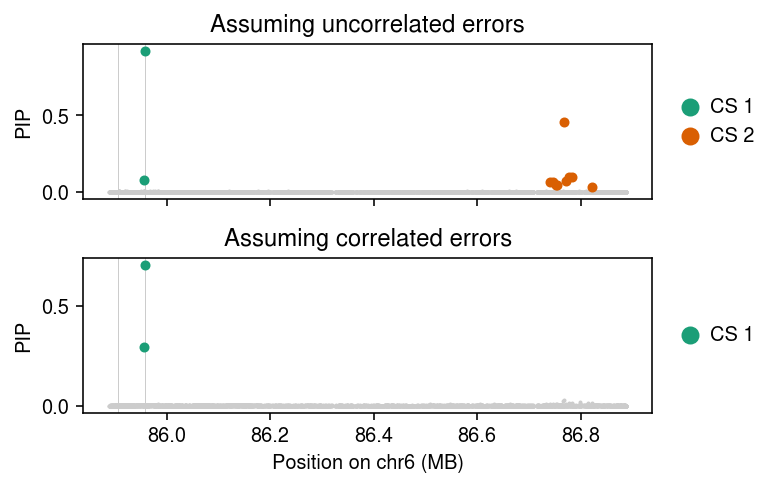
Plot the estimated PIPs under each fitted model, highlighting the credible sets. Mark the simulated causal variants by vertical lines.
cm = plt.get_cmap('Dark2')
pos = np.array([float(t[-1]) / 1e6 for t in x.columns.str.split('_')])
plt.clf()
fig, ax = plt.subplots(2, 1, sharex=True)
fig.set_size_inches(5.5, 3.5)
for a, fit in zip(ax, [fit0, fit1]):
  a.scatter(pos, np.array(susie.susie_get_pip(fit)), s=1, c='0.8')
  temp = susie.susie_get_cs(fit, X=xs).rx2('cs')
  if temp:
    cs = [np.array(c) - 1 for c in temp]
    for i, c in enumerate(cs):
      a.scatter(pos[c], np.array(susie.susie_get_pip(fit))[c], s=16, c=cm(i), zorder=3, label=f'CS {i+1}')
  a.legend(frameon=False, markerscale=2, handletextpad=0, loc='center left', bbox_to_anchor=(1, .5))
  a.set_ylabel('PIP')
  for p in np.where(b != 0)[0]:
    a.axvline(pos[p], c='0.8', lw=0.5, zorder=2)
ax[0].set_title('Assuming uncorrelated errors')
ax[1].set_title('Assuming correlated errors')
ax[-1].set_xlabel('Position on chr6 (MB)')
fig.tight_layout()
Related work
Schelldorfer et al. 2011 consider a model in which \(\vb\) is \(\ell_1\)-penalized rather than assuming a sparsity-inducing prior on \(\vb\). The approach they take is to make coordinate updates to the variance components, using exact gradient and approximate Hessian information, and is implemented in the R package glmmlasso.
Peter Carbonetto showed how to reduce BSLMM (Zhou et al. 2013) to varbvs (Carbonetto and Stephens 2012) using this approach.
Zhengyang Fang incorporated the BSLMM prior into susie using this approach, implemented in susie-mixture. However, their approach assumes \(\mk\) depends on the same cis-genotypes as the design matrix \(\mx\), leading to severe inference problems related to proximal contamination. In contrast, we are motivated by the case where \(\mk\) depends on the rest of the genome.
Andrew Goldstein generalized susie to the exponential family (generalized linear models) using this approach.